Specifying demographic model with structure
GADMA infers a demographic model from an AFS with nothing required from the user, except for simple information that determines how much the detailed model is required - the structure of the model.
Warning
This feature is available only up to three populations. If there is more than three populations then unfortunately only custom model could be used alongside with Bayesian optimization instead of genetic algorithm. More information about demographic inference for four and five populations please see here.
Assume a division of one population into two new subpopulations and a fixed temporal order of the populations: from the most anciently to the most recently formed population.
We can divide time of our model into split events and time intervals, during which a certain dynamics of change of effective size is maintained for each population and migration rates are constant. The number of split events is one less than the number of populations under consideration. Now we can define the concept of the structure of the demographic model:
- The structure of the demographic model is:
the number of time intervals in case of one population;
the numbers of time intervals before and after a single split, in the case of two populations;
the numbers of time intervals prior to the first split, between the two splits, after the second split, in the case of three populations.
Example of representation of demographic model. Time is on the axis of abscissa and population size is on the axis of ordinates. The structure of that model is (2,1,1). The colours reflect different demographic dynamics:
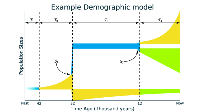
For example, we can divide the time of the model on the figure above to four time intervals: T1, T2, T3 and T4, and two population splits: S1 and S2. The structure of this model is (2, 1, 1) because two intervals (T1 as T2) before first split S1, one interval (T3) between first and second splits and one interval (T4) after second split S2.
Initial structure
To specify the structure of the inferred model one should set Initial structure in the parameter file:
# param_file
...
Initial structure : 2
...
or
# param_file
...
Initial structure : 2,1
...
or
# param_file
...
Initial structure : 2,1,1
...
By default the simplest structure is used (1 or 1,1 or 1,1,1).
Final structure
It is also possible to start with a simpler structure in order to get to a more complex one. The runs with different Initial structure and Final structure will find models with small number of parameters first and increase that number to achieve final structure. Such pipeline will take more time resources but the result is more stable. To do so one should specify option Final structure in the parameter file. For example:
# param_file
Input data : some_2d_fs.fs

Initial structure : 1,1
Final   structure : 2,1
...
Within this parameter file GADMA will find parameters for demographic model with 1,1 structure, then increase the structure to 2,1 and find parameters for the model with this structure. Parameters identified within a more simple structure (in this case it is 1,1) are used further to define the parameters of a more complex structure (2,1).
Note
The initial structure is transformed to the final structure in a number of steps, each corresponding to the increment of one component by one. If there is more than one component to increment, the actual incremented component will be selected randomly, so if one specifies initial structure to 1,1 and final to 2,2, it is not guaranteed to final optimal parameters for demographic models with structures between 1,1 and 2,2, i.e. intermediate state can be either 1,2 or 2,1.
Warning
Use the scheme with a more complex structure, as it produces more stable solutions.
Warning
Choose the recommended values for model structure. The final structure should differ from initial structure only by one element , for example, 1,1 and 2,1; 1,2,1 and 2,2,1.
Additional options
Dynamics of size change
Three main demographic dynamics of population size change:
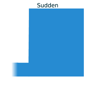
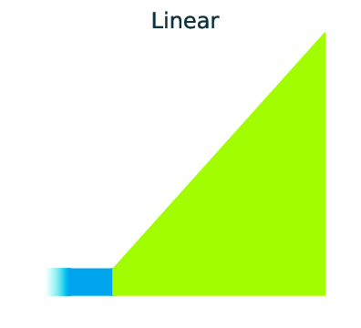
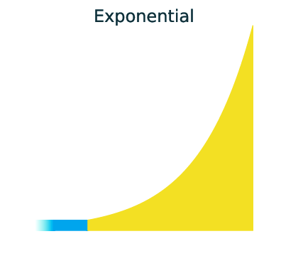
In GADMA the size of population can be changed due to one of three dynamics: sudden change, linear change and exponential change of the effective population size.
In order to infer a demographic model with sudden changes of populations sizes only, option Only sudden in the parameters file should be set to True:
# param_file
...
Only sudden : True
...
By default, this option is set to False and dynamics are found like other parameters of the demographic model.
It is also possible to disable some dynamics by setting Dynamics option to allowed values. For example, to exclude linear size change:
# param_file
...
Dynamics : Sud, Exp
...
Inbreeding
GADMA can estimate inbreeding coefficients for demographic models with structure using dadi engine. To enable inbreeding coefficients one should set the following:
# param file
...
Inbreeding: True
...
No migrations and symmetric migrations
GADMA can exclude migrations rates from optimization and consider them equal to zero. In that case all migrations are disabled. One should set option No migrations to True in the parameter file.
To estimate symmetric migrations one should set Symmetric migrations to True.
# param file
...
No models: False
Symmetric migrations: True
...
Restrict some migrations
It is possible to restrict some number of migrations by setting the Migration masks option. It is a list of masks for each time interval after first split.
For example, if there is model structure equal to (2, 1, 1) and one want to have all zero migrations except (a) migration from population 1 to population 2 between split of ancestral population and second split and (b) migration between population 1 and population 3 after second split. Then for first interval after split mask will be [[None, 0], [1, None]] (m[i, j] corresponds to the migration from the population j to the population i) and for next time interval right after the second split mask will be [[None, 0, 1], [0, None, 0], [1, 0, None]].
# params_file
Migration masks: [[[0, 0], [1, 0], [[0, 0, 1], [0, 0, 0], [1, 0, 0]]]
Note
Option Migration masks is used only in case of demographic model with structure and Initial structure equal to Final structure.
Note
When option Migration masks is used together with Symmetric migration masks should be symmetrical. There is no such option to make some migrations symmetrical and other not.
Selection and dominance coefficients
To enable inference of selection coefficients in demographic history set option Selection to True:
# param file
...
Selection: True
...
It is posiible to infer dominance coefficients also:
# param file
...
Selection: True
Dominance: True
...
Split fractions
Split could be set in two ways:
Population is split according to some
fraction:size * fractionbecomes size of first subpopulation andsize * (1 - fraction)becomes the size of the second subpopulation. In this case sizes of newly formed populations could not be greater than the size of their parent population.Sizes of newly formed subpopulations are independent from the size of the parent population. In that case the demographic model will have one additional one parameter per each split in it compared to the model from the first point.
# param file
Split fractions: True  # for 1) point
Upper and lower bounds of splits
It is possible to limit time of split events in the demographic model with structure. In order to do that one should specify one or multiple options in the parameter file that refer to lower and upper bounds of split events. Splits are numbered from the most ancient, so split 1 is a split event that occurred with the ancient population and split 2 is the next division of the second population (exist only for three populations). There are three options corresponded to split times: Lower bound of first split, Upper bound of first split, Lower bound of second split and Upper bound of second split.
Bounds should be specified in GENERATIONS. In order to translate time from years to generations, divide it by T_g, where T_g is time (in years) for one generation. For example, assume we want the last split to be between 1000 and 2000 years. Time for one generation is estimated to be 24 years. Therefore we construct the following parameter file:
   # param_file
   ...
   Lower bound of second split : 41.666
   Upper bound of second split : 83.333
   ...

It is allowed to set any of those four options, just make sure they make sense. It is possible to set only one bound or one lower and one upper bounds for different splits:

.. code-block:: none

   # param_file
   ...
   # In that particular case upper bound for the second split exists automatically
   Upper bound of first split : 30
   Lower bound of second split : 10
   ...