Inference for four and five populations

Demographic inference for four and five populations is time-consuming. GADMA offers special algorithm for that case - Bayesian optimization. Here we show how to run Bayesian optimization within GADMA framework on example dataset of four populations.

Dataset

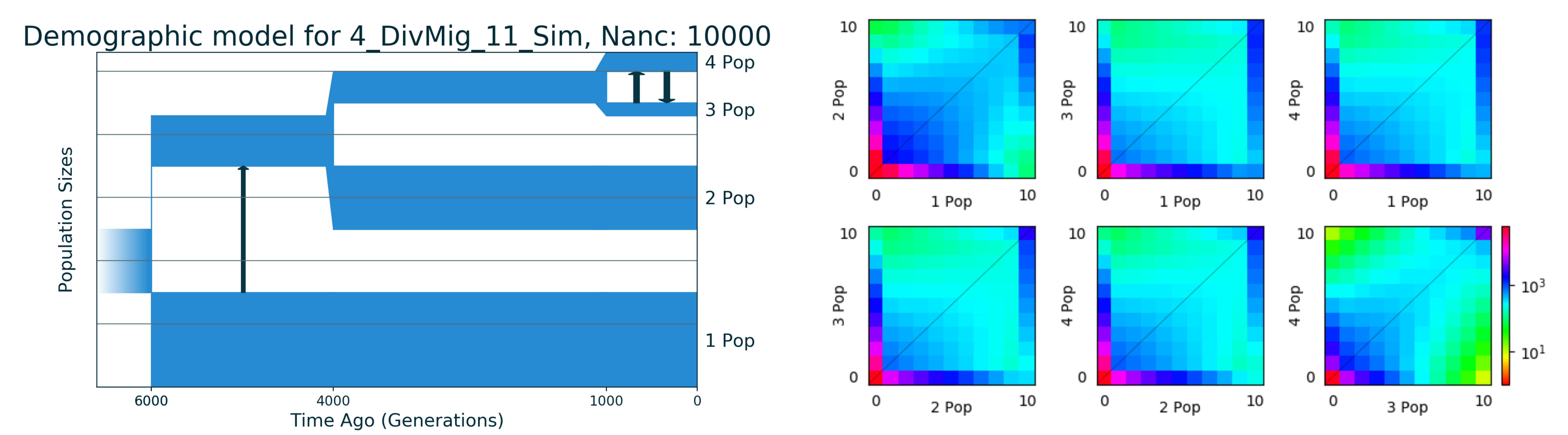
The dataset we will use is simulated dataset for four populations named 4_DivMig_11_Sim from `deminf_data <https://github.com/noscode/demographic_inference_data>`__. The description of its eleven parameters could be found in the repository of deminf_data package given above.

We should hightlight here the best known value of log-likelihood: -16932.827. The data and demographic model are stored in the data_and_model directory. The picture of the best model and simulated SFS data could be found below:

from IPython.display import Image
from IPython.core.display import HTML

Image("4_DivMig_11_Sim_picture.png")

Using Bayesian optimization ensemble for demographic inference

In order to run Bayesian optimization approach instead of genetic algorithm one should use setting Global optimizer: SMAC_BO_combination. It will run ensemble approach that showed best performance. It is also recommended to set Num init const to the value of 2 as it will decrease number of points generated by initial design. Setting Global maxeval corresponds to the maximum number of evaluations in optimization and is required in case of Bayesian optimization. We run 200 evaluations, maximum recommended number is 400.

!cat bo_ensemble_params

Input file: data_and_model/fs_data.fs
Output directory: bo_combination
Custom filename: data_and_model/demographic_model.py

Num init const: 2
Global optimizer: SMAC_BO_combination
Global maxeval: 200

Number of repeats: 64
Number of processes: 8

To run GADMA:

!gadma -p bo_ensemble_params

Results

We have run BO ensemble and the results are presented in bo_combination directory. Top 10 best models:

!tail -81 bo_combination/GADMA.log | head -13

[030:40:12]
All best by log-likelihood models
Number  log-likelihood  Model
Run 35  -16989.04       (nu1=1.51436,   nu234=1.21784,  nu2=0.91519,    nu34=0.43356,   nu3=0.21684,    nu4=0.33271,    m12_anc=0.00656,        m34_sym=0.23666,        T1=0.11024,     T2=0.14063,     T3=0.03952)     f
Run 37  -17035.23       (nu1=1.4675,    nu234=0.70827,  nu2=1.02063,    nu34=0.59681,   nu3=0.14219,    nu4=0.21247,    m12_anc=2.98575,        m34_sym=0.00086,        T1=0.10249,     T2=0.18656,     T3=0.0248)      f
Run 15  -17046.36       (nu1=1.50765,   nu234=0.76371,  nu2=1.01515,    nu34=99.80705,  nu3=0.20986,    nu4=0.28198,    m12_anc=0.10372,        m34_sym=6.21095,        T1=0.07263,     T2=0.00468,     T3=0.20416)     f
Run 28  -17061.33       (nu1=1.56268,   nu234=1.17196,  nu2=1.00151,    nu34=0.38991,   nu3=0.28053,    nu4=0.35989,    m12_anc=0.77758,        m34_sym=3.13455,        T1=0.12101,     T2=0.11256,     T3=0.07957)     f
Run 13  -17064.24       (nu1=1.42257,   nu234=0.40176,  nu2=1.05118,    nu34=0.56015,   nu3=0.22039,    nu4=0.31252,    m12_anc=3.84063,        m34_sym=3.93956,        T1=0.04597,     T2=0.14905,     T3=0.07111)     f
Run 24  -17074.33       (nu1=1.55419,   nu234=0.83564,  nu2=1.04965,    nu34=0.44669,   nu3=0.21901,    nu4=0.3659,     m12_anc=1.18466,        m34_sym=1.92174,        T1=0.09211,     T2=0.15544,     T3=0.0518)      f
Run 5   -17094.97       (nu1=1.52389,   nu234=1.35875,  nu2=0.95452,    nu34=0.23971,   nu3=0.20094,    nu4=0.28331,    m12_anc=0.00203,        m34_sym=6.35301,        T1=0.12177,     T2=0.00777,     T3=0.17876)     f
Run 60  -17119.19       (nu1=1.59878,   nu234=1.26844,  nu2=1.03675,    nu34=0.579,     nu3=0.11958,    nu4=0.19174,    m12_anc=0.08318,        m34_sym=0.0065, T1=0.10808,     T2=0.19021,     T3=0.02171)     f
Run 30  -17133.73       (nu1=1.5429,    nu234=0.58485,  nu2=1.13619,    nu34=0.64745,   nu3=0.19726,    nu4=0.32858,    m12_anc=3.3243, m34_sym=3.67529,        T1=0.07238,     T2=0.1914,      T3=0.0497)      f
Run 34  -17139.85       (nu1=1.27549,   nu234=0.51191,  nu2=1.04419,    nu34=0.50946,   nu3=0.14838,    nu4=0.21779,    m12_anc=1.07316,        m34_sym=1.1489, T1=0.05095,     T2=0.17626,     T3=0.02714)     f

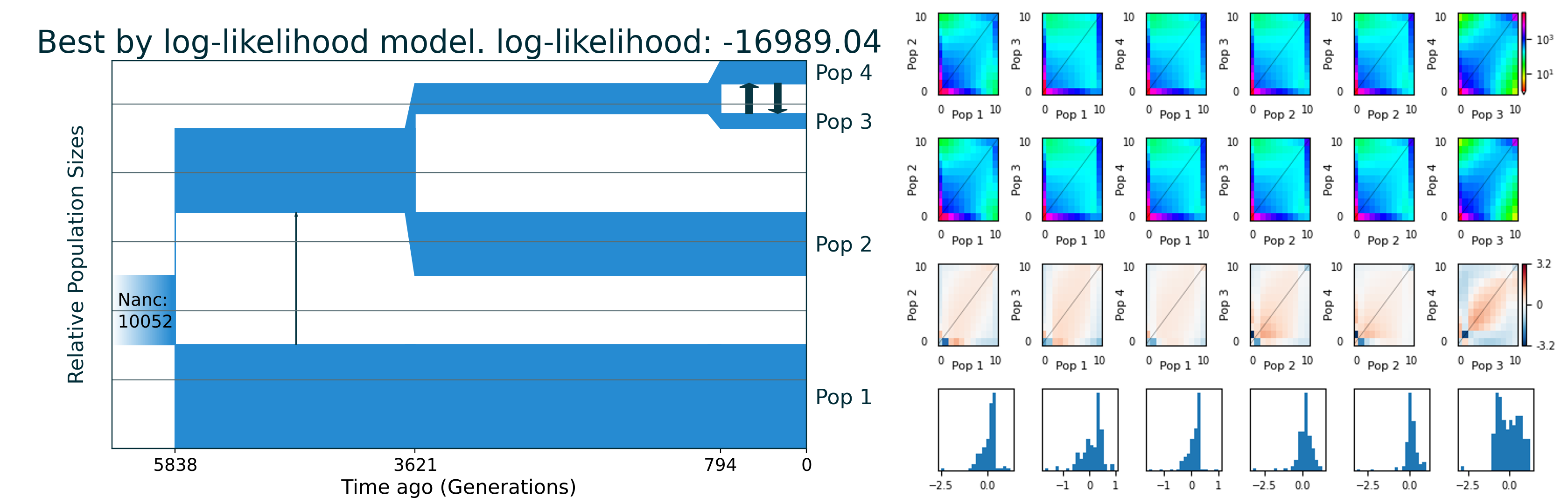
The best demographic model has log-likelihood -16989.04. It is close to the optimum value. The result model:

Image("bo_combination/best_logLL_model.png")

Other Bayesian optimization available options

GADMA has several Bayesian optimizations. The first one is vanilla BO (SMAC_BO_optimization), it is possible to set prior choice via Kernel and acquisition function via Acquisition function for it.

!cat bo_vanilla_params

Input file: data_and_model/fs_data.fs
Output directory: bo_combination
Custom filename: data_and_model/demographic_model.py

Num init const: 2

Global optimizer: SMAC_BO_optimization
# Choice of prior for Gaussian process
# Could be: exponential, Matern32, Matern52, RBF
Kernel: matern52
# Choice of acquisition function for BO
# Could be: EI, PI, logEI
Acquisition function: PI

Global maxeval: 200

Number of repeats: 64
Number of processes: 8

The last algorithm based on Bayesian optimization in GADMA is BO with automatic prior selection. In order to change to this pipleine setting Kernel should be set to auto:

!cat bo_auto_params

Input file: data_and_model/fs_data.fs
Output directory: bo_combination
Custom filename: data_and_model/demographic_model.py

Num init const: 2

Global optimizer: SMAC_BO_optimization
# If auto then automatic prior selection
Kernel: auto
Acquisition function: PI

Global maxeval: 200

Number of repeats: 64
Number of processes: 8